10 COMPONENTS
A component is a self-contained software building block with a well-defined interface with its outside world.
In this chapter we will start with a description of how software components are structured. Then we will discuss the interactions between different components and how to use components.
A software component is designed to perform a number of related functions. It consists of two parts:
1. the interface-section, which contains the signatures of all the operations and functions which may be called from outside the component. Additionally, it may also contain type-specifications.
2. the implementation-section, which contains the definitions of the operations and functions which are externally accessible as specified in the interface-section. It may also contain other definitions which are local to the component.
To illustrate the structure and use of components, let us assume that we want to create and manipulate two-dimensional graphical figures which are made from simple geometric objects such as points, triangles, circles. Let us also assume that the only operations on those figures are to create a figure, to move (translate) a figure, to enlarge (scale) a figure and to rotate a figure. Let's first start with a component for two-dimensional Points ( Figure 10-1):
component Points;
 type Point;
      Point ( X_coord = Numeric, Y_coord = Numeric ) -> Point;
      Abscissa ( Point ) -> Numeric;
      Ordinate ( Point ) -> Numeric;
      Translate ( Point, NewOrigin = Point ) -> Point;
      Scale ( Point, Factor = Numeric )	-> Point;
      Rotate ( Point, Angle = Numeric ) -> Point;
begin
      Point (x, y) = Point:[ x; y ];
      Abscissa (P) = P.x;
      Ordinate (P) = P.y;
      Translate (P, S)	= Point ( P.x + S.x, P.y + S.y );
      Scale (P, f) = Point ( f * P.x, f * P.y );
      Rotate (P, a) = Point ( P.x * cos (a) + P.y * sin (a),
                             -P.x * sin (a) + P.y * cos (a) );
end component Points;
Figure 10-1: Example of a component for two-dimensional points
As is shown by this example, a component starts with a line, containing the name of the component, and it ends with an end component line, also mentioning the component name. As a convention, we will name the component after the type or the functions it represents: in case of type we will often use the type name in plural.
The interface-section of a component starts after the first line and it ends with the line containing the word 'begin'. In our example, the interface-section introduces Point as the name of a new descriptor type and it lists the signatures of six operations defined on points. The first operation will introduce the two coordinate values of a new Point. Both are of type Numeric. For the time being we will assume that Numeric types are representing integer numbers. The second operation will return the x-coordinate of a given point. The third operation will return the y-coordinate of a given point. The fourth operation will move a given point relative to the new origin of the coordinate system. The fifth operation will multiply the x-coordinate and the y-coordinate of a point with the given scaling factor. The last operation will rotate a point through a clockwise angle about the origin of the coordinate system.
With the Point specification we are now able to describe points and to define compound operations on points. Some examples are:
Point (25, 47)Translate (Point (30, 47), Point (5, 7))Ordinate (Scale ( Point(-31, -55), 2 ))Point (Ordinate (Point (2, 3)), Abscissa (Point (2, 3)))
The implementation-section of a component starts after the line with the word 'begin' and it ends with the last line of the component. In our example, it contains definition rules which are in one to one correspondence with the specifications in the interface-section.
The first definition rule in the implementation-section corresponds to the constructor operation for a new Point. It will create with each invocation a new Point-descriptor - denoted by Point:[ x; y] - with the values of the x- and the y-coordinates.
The following lines are definition rules corresponding with the operations specified on Point objects. For instance, the Abscissa operation will return the value of the x-coordinate of the input Point by reading the x value in the corresponding Point descriptor. Similar, the Ordinate operation will return the value of the y-coordinate. The Translate operation will add the values of the corresponding entries of the input descriptors and will create a new Point descriptor with the new values. The Scale and Rotate operations also have their corresponding definitions.
Exercise:
- 10.1 Make a component for points in three-dimensional space.
In general, a component provides a number of services to its clients. A client may be a human being taken part in a dialog session, it may be a program, or it may be another component. All those users are clients of the component. Clients request services by issuing requests. Requests are events that occur during the execution of the program. A request is honored by the execution of a definition call.
The services a component provides are specified in its interface-section. The definitions of an implementation-section are not accessible for a client, except through the services provided by the interface. That means that descriptors, their elements, and the related definitions are encapsulated in a component. The main reason for encapsulation, or, equivalently information hiding, is that the internal definitions in the implementation-section can be changed without changing the interface. That means that as long as the interface-section has not been changed, a client may continue to use such a component without adapting its program.
10.3 Relations between Components
A component may be based on other components. To illustrate the relationships between components we will use as an example a component for Triangles (Figure 10-2) based upon the already defined Points component:
component Triangles;
 type Triangle;
      Triangle ( Point, Point, Point ) -> Triangle;
      Translate ( Triangle, NewOrigin = Point)	-> Triangle;
      Scale ( Triangle, Factor = Numeric )	-> Triangle;
      Rotate ( Triangle, Angle = Numeric )	-> Triangle;
begin
      Triangle (P1, P2, P3) = Triangle:[ P1; P2; P3 ];
Translate (T, p) = Triangle (Translate (T.P1, p ), Translate (T.P2, p ), Translate (T.P3, p ));Scale (T, f) = Triangle (Scale (T.P1, f ), Scale (T.P2, f ), Scale (T.P3, f ));Rotate (T, a) = Triangle (Rotate (T.P1, a ), Rotate (T.P2, a ), Rotate (T.P3, a )); end component Triangles;
Figure 10-2: Example of a component for triangles
This component is similar in structure as the Point component. The specification in the interface-section states that a Triangle is characterized by its type and three entities, which are representing the corner points of a triangle. These entities must be objects of type Point as introduced in the interface-section of the previous component. So, the Triangle component is built on top of the Point component.
The operations Translate, Scale and Rotate are similar to the corresponding operations defined for Points. They are transforming Triangles into other Triangles. We will not discuss them in detail. Of course, also compound operations can be defined on Triangles.
The first definition rule in the implementation-section contains the descriptor-constructor for Triangles. The Triangle-descriptor Triangle:[P1; P2; P3] has three entries: one for each corner point.
The three remaining definition rules are all very similar in nature. They are all using the corresponding operations of the Points component. Take for example the Translate definition: What it does is very simple: it translates the three corner-points and then returns a new triangle with the translated corner-points. The same applies to the Rotate and Scale definitions.
So, here we see the interaction between the Triangles component and the Points component. May be you would ask the question: How does Elisa knows when Point operations should be used? That is because it uses the method of type propagation we discussed earlier to determine the type of each entity in a component.
Let us start in our example with the definition containing the Triangle-descriptor. The types of the input items of this definition are Points as specified in the interface section, and therefore the entries in the Triangle-descriptor are also of type Points.
In the following definition the Translate operation has two parameters, the first is of type Triangle, the second is of type Point. In this definition three Translate operations are specified: each one selects from the given Triangle-descriptor a Point and as a result of type propagation the three Translate operations all have arguments of type Point and are therefore referring to the operation:
Translate (Point, Point)
Because this matches with the corresponding operation given in the interface-section of the Points component, the Translation of a Point will be applied.
Exercise:
- 10.1 Make a component for triangles in three-dimensional space.
10.4 Evaluation of Descriptor Expressions
Based on our understanding of the relationships between different components we are now able to show the evaluation of compound expressions involving descriptors. Therefore we will use a component for Circles as defined in the followings (Figure 10-3):
component Circles;
 type Circle;
      Circle (Center = Point, Radius = Numeric ) -> Circle;
      Translate ( Circle, NewOrigin = Point)	 -> Circle;
      Scale ( Circle, Factor = Numeric )	 -> Circle;
      Rotate ( Circle, Angle = Numeric )	   -> Circle;
begin
      Circle (Center, Radius) = Circle:[ Center; Radius ];
      Translate (C, P)	= Circle (Translate (C.Center, P), C.Radius);
      Scale (C, f) = Circle (Scale (C.Center, f), f * C.Radius);
      Rotate (C, a) = Circle (Rotate(C.Center, a), C.Radius);
end component Circles;
Figure 10-3: Example of a component for circles
This example shows us a descriptor with elements of different types: the Circle-descriptor Circle:[ Center; Radius] contains a Point and a Numeric element.
The operations Translate, Scale and Rotate are similar to the corresponding operations defined for Points. They are transforming Circles into other Circles. They are also making use of the corresponding operations defined for Points. We will not discuss them in detail.
To get more insight in the implications of defining components on top of other components, we will follow in detail the evaluation of a compound expression based on the Circles and Points components. Suppose we want to evaluate the following expression:
Scale (Translate (Circle (Point (2, 5), 17), Point (13, 19)), 3)
Or, if we express this in words: Given a circle with center-point (2,5) and a radius of 17; translate the circle with respect to the new origin (13,19) and scale the translated circle with a factor 3. For this exercise we assume that type Numeric is equivalent to the predefined type integer.
As a rule, we will always evaluate a compound expression by evaluating successive sub-expressions going from the inside to the outside of the expression. So, by evaluation and substitution of the first and second Points we get two Point-descriptors in:
Scale (Translate (Circle (Point:[ x=2; y=5], 17), Point:[ x=13; y=19]), 3)
Evaluating the Circle-expression gives us a Circle-descriptor in:
Scale (Translate (Circle:[ Center= Point:[x=2; y=5]; Radius=17], Point:[ x= 13, y= 19] ), 3)
Substitution of the Translate definition for Circles gives us:
Scale (Circle (Translate (Point:[ x=2; y=5], Point:[ x=13; y=19], 17), 3)
Substitution of the Translate definition for Points results in:
Scale (Circle (Point (15, 24), 17), 3)
Substitution of the Point expression gives us a Point-descriptor:
Scale (Circle (Point:[ x=15; y=24 ], 17), 3)
Evaluating the Circle expression gives us a Circle-descriptor:
Scale (Circle:[ Center= Point:[ x= 15; y= 24 ]; Radius=17 ], 3)
Substitution of the Scale definition for Circles gives us:
Circle (Scale (Point:[ x= 15; y= 24], 3), 3 * 17)
Substitution of the Scale definition for Points gives us:
Circle (Point (45, 72), 51)
Substitution of the Point expression gives us a Point-descriptor:
Circle (Point:[ x= 45; y= 72], 51)
Evaluating the Circle expression gives us a Circle-descriptor:
Circle:[ Center= Point:[ x= 45; y= 72]; Radius= 51]
And this is the end of the evaluation. This expression cannot be reduced any further. So, the evaluation of the original compound expression results in an object of type Circle with the center point (45,72) and a radius of 51.
The main reason we did this exercise, was to make you aware of the many detailed steps involved in the evaluation of compound expressions, even with the very simple definitions as given in our examples. Fortunately, this substitution process can be performed in a mechanical way and can therefore much better be done by a computer.
Exercise:
- 10.3 Follow the evaluation, step by step, of the expression
Scale (Circle (Point (7, 3), 13), 5).
- 10.4 Make a component for spheres in three-dimensional space.
In one of the previous sections we discussed how compound descriptor-expressions are evaluated. Our examples were based on one descriptor per operand. However, as we discussed earlier, expressions may also represent multiple entities. So, we will illustrate how expressions can represent streams of descriptors. We will give some examples based on our graphical components.
Our first example is to define a sequence of concentric circles. The expression representing such a sequence is very simple using our previously defined Circles component:
Circle (Point (3, 3), 1 .. 7)
The evaluation of this expression creates a stream of 7 concentric circles all with the center point(3,3). The first element of the stream is the most inner circle with a radius of 1, the second is a circle with a radius of 2, the third with 3 etc. The last element of the stream is the most outer circle with a radius of 7.
We also could have written the expression in another way:
[ C = Point (3, 3); R = 1 .. 7; Circle (C, R) ]
This expression block has the same effect as the expression; the only difference is that we assigned local names to the sub-expressions
Up to now it was simple: we had only a fixed number of objects in a stream. But suppose that we want to define a stream with a variable number of concentric circles around any center point. The following definition will do:
ConcentricCircles (Point, Number = integer) -> multi (Circle);
ConcentricCircles (P, N) = Circle (P, 1 .. N);
What happens if we issues the call ConcentricCircles (Point (1, 2), 5)? The definition will return a stream of 5 Circle-descriptors which are concentric around Point(1,2). This example shows us how a definition may produce a stream of descriptors.
Exercises:
- 10.5 Make a definition of concentric circles where all center points are on equal distances from the x and the y axes.
- 10.6 Make a definition of concentric spheres in three-dimensional space.
In the preceding sections we have seen how software components are constructed. However, we did not discuss how they could be selected. We simply assumed they were there. In practice, software components are stored in so-called libraries. A library of software components contains all those software components which are used by a set of related applications. If we now want to use a component, we simply give the word use, followed by the component-name. In our examples of geometric components, we can select those components by the following use directives:
use Points;
use Triangles;
use Circles;
The use directives are making the specified components available for further use. Multiple components may be used in one use directive. So, the three use directives may also be written as:
use Points, Triangles, Circles;
After some components have been programmed, the question is: how are we verifying those components? Or, in other words, are the basic operations as implemented by a component functioning according to the specifications given in the interface-section and according to our expectations.
As an illustration we will verify in a session the components of our geometric objects as defined in this chapter. We want to start with the Points component. However, because the Points component makes use of a Numeric type we first need to define what that is. We have assumed already that the type Numeric is equivalent to the built-in type integer. So, we are beginning our session with:
type Numeric = integer;
use Points;
Point (23, 45)?
The first reaction of the system will be that the sine and cosine functions - used in the Rotate definition of the Point component - are not defined for integer numbers. That means that our assumption that type Numeric could be substituted by type integer was wrong! So, this is the first, although negative, result of our verification effort. Now we have to make a choice. Either we are adapting the Point component or we assume that type Numeric may be equivalent to the built-in type real, because we know that the sine and cosine functions are defined for reals. We decide for the second option. So, we start a new session with:
type Numeric = real;
use Points;
Point (23.0, 45.0)?
This request is accepted and the system returns with the answer:
Point:[ x = 23.0; y = 45.0]
We may further interrogate the Points component via its interface, as shown in the following:
Abscissa (Point (-5.0, -7.0))?
-5.0
Translate( Point (3.3, 5.5), Point (6.0, 10.0))? Point:[ x = 9.3; y = 15.5]Scale (Point (-3.5, 6.8), 2.0)? Point:[ x = -7.0; y = 13.6]Rotate (Point (4.0, 9.0), 3.14159265359)? << 180 degrees >> Point:[ x = -4.0; y = -9.0]
Let us assume that after a number of tests we are satisfied with the behavior of our Points component and we want to verify another component in our hierarchy. We decide for the Triangle and we start a new session:
type Numeric = real;
use Points, Triangles;
P1 = Point (4.0, 9.0);
P2 = Point (6.0, -3.0);
P3 = Point (-5.0, 7.0);
T1 = Triangle (P1, P2, P3);
T1?
The system returns with:
Triangle:[ P1 = Point:[x = 4.0; y = 9.0];
           P2 = Point:[x = 6.0; y = -3.0];
           P3 = Point:[x = -5.0; y = 7.0]]
We continue with the dialogue:
T2 = Translate (T1, Point (5.0, 5.0));
T2?
Triangle:[ P1 = Point:[x = 9.0; y = 14.0];
           P2 = Point:[x = 11.0; y = 2.0];
           P3 = Point:[x = 0.0; y = 12.0]]
Scale (T2, 3.0)? Triangle:[ P1 = Point:[x = 27.0; y = 42.0]; P2 = Point:[x = 33.0; y = 6.0]; P3 = Point:[x = 0.0; y = 36.0]]Rotate (T1, 3.14159265359)? << 180 degrees >> Triangle:[ P1 = Point:[x = -4.0; y = -9.0]; P2 = Point:[x = -6.0; y = 3.0]; P3 = Point:[x = 5.0; y = -7.0]]
After the Triangles component has been verified, we may continue with the Circles component. Because it is quite similar to the previous session we will not discuss it here.
After all the relevant components are verified in this way we may compose a system out of the components. One of the goals is to investigate how the system behaves for different inputs and under several conditions. In essence, we will use the same techniques as described in previous sessions.
We will use as an example two-dimensional figures based on the verified components. For the sake of simplicity we assume that a figure consists of a head, represented by a circle, and a body, represented by a triangle. The corresponding component is defined as follows (Figure 10-4):
component Figures;
 type Figure;
      Figure ( Head = Circle, Body = Triangle )	-> Figure;
      Translate ( Figure, NewOrigin = Point ) -> Figure;
      Scale ( Figure, Factor = Numeric ) -> Figure;
      Rotate ( Figure, Angle = Numeric ) -> Figure;
begin
      Figure (Head, Body) = Figure:[ Head; Body ];
Translate (F, P) = Figure (Translate (F.Head, P ), Translate (F.Body, P));Scale (F, f) = Figure (Scale (F.Head, f ), Scale (F.Body, f));Rotate (F, a) = Figure (Rotate (F.Head, a ), Rotate (F.Body, a)); end component Figures;
Figure 10-4: Example of a component for figures
Our system can now be assembled in the following way:
type Numeric = real;
use Points, Triangles, Circles, Figures;
Now we may use our system in various ways. As an example we will create a small puppet and then use that for some manipulations:
P1 = Point (3.0, 4.0);	P2 = Point (2.0, 1.0); P3 = Point (4.0, 1.0);
Body = Triangle (P1, P2, P3);
Head = Circle (Point (3.0, 5.0), 1.0);
Puppet = Figure (Head, Body);
Puppet?
The system will answer with:
Figure:[ Head= Circle:[ Center= Point:[x = 3.0; y = 5.0]; Radius = 1.0];
         Body= Triangle:[ P1 = Point:[x = 3.0; y = 4.0];
                          P2 = Point:[x = 2.0; y = 1.0];
                          P3 = Point:[x = 4.0; y = 1.0]]]
On this Figure we will put some operations into action:
Translate (Puppet, Point (5.0, 3.0))?
Figure:[ Head = Circle:[Center = Point:[x = 8.0; y = 8.0]; Radius = 1.0];
         Body = Triangle:[P1 = Point:[x = 8.0; y = 7.0];
                          P2 = Point:[x = 7.0; y = 4.0];
                          P3 = Point:[x = 9.0; y = 4.0]]]
Rotate (Puppet, 3.14159265359 / 2.0)? << 90 degrees >> Figure:[ Head = Circle:[Center = Point:[x = 5.0; y =-3.0]; Radius = 1.0]; Body = Triangle:[P1 = Point:[x = 4.0; y = -3.0]; P2 = Point:[x = 1.0; y = -2.0]; P3 = Point:[x = 1.0; y = -4.0]]]
The results of the Translate and Rotate operations are shown in the preceding data. Although many other combinations of operations can be tested, we will not do that. Essential is to understand how operations can be defined on compound objects and how they can be tested interactively.
10.8 Mutable and Immutable Objects
In the components of Points, Triangles, Circles, and Figures we only used constructor and accessor operations; no mutators were used. As a consequence, descriptors of these types could not be modified. We say that those descriptors are immutable. This is in contrast to mutable descriptors, such as, for instance, the Employee descriptor defined in the preceding chapter where we were allowed to change the salary of an Employee. Mutable descriptors are often used to represent the current state of their real life counterparts. For example, changing the salary of an Employee will change the state of the Employee record correspondingly.
Because for immutable descriptors no mutators are defined, the state of those descriptors cannot be changed. Consequently, immutable descriptors are not altered; they remain as they are at creation time. When needed, a new descriptor will be created. For example, the translation of a Point is not defined by changing the coordinates of the original Point, but by creating a new Point with the new coordinates. The original Point remains unaffected and can be reused in other computations.
Let us investigate what the differences are between immutable and mutable descriptors. For example, let us start with defining a component for mutable Points (see Figure 10-5).
component MutablePoints;
 type Point;
      Point (X_coord = Numeric, Y_coord = Numeric ) -> Point;
      Abscissa ( Point ) -> Numeric;
      Ordinate ( Point ) -> Numeric;
      Translate ( Point, NewOrigin = Point ) -> Point;
      Scale ( Point, Factor = Numeric ) -> Point;
      Rotate ( Point, Angle = Numeric ) -> Point;
begin
      Point (x, y) = Point:[ x; y];
      Abscissa (P) = P.x;
      Ordinate (P) = P.y;
      Translate (P, S) = [ P.x:= P.x + S.x; P.y:= P.y + S.y; P];
      Scale (P, f) = [ P.x:= f * P.x; P.y:= f * P.y; P];
      Rotate (P, a) = [ P.x:= P.x * cos(a) + P.y * sin(a);
                        P.y:=-P.x * sin(a) + P.y * cos(a); P];
end component MutablePoints;
Figure 10-5: Example of a component for two-dimensional mutable points
Compare this component with the original component for Points. The interface sections of both components are the same. However, the Translate, Scale, and Rotate operations are changed into mutator operations.
Let us use this component in the following session:
type Numeric = real;
use MutablePoints;
P1 = Point (4.0, 9.0); P1? Point:[x = 4.0; y = 9.0]
This is according to our expectations, because the constructor operation has not been changed. But what happens if we use one of the mutator operations?
Scale (P1, 3.0)?
Point:[x = 12.0; y = 27.0]
The Scale operation gives the expected result. But what happened to the original Point P1?
P1?
Point:[x = 12.0; y = 27.0]
It turns out that P1 has also been changed. The reason is that, although P1 still refers to the original Point-descriptor, the values of the descriptor elements have been changed by the Scale operation.
Let us now use a more complicated example by using this component in combination with the unchanged Triangles component:
type Numeric = real;
use MutablePoints, Triangles;
P1 = Point (1.0, 1.0);
P2 = Point (7.0, 1.0);
P3 = Point (4.0, 4.0);
T1 = Triangle (P1, P2, P3); T1? Triangle:[ P1 = Point:[x = 1.0; y = 1.0]; P2 = Point:[x = 7.0; y = 1.0]; P3 = Point:[x = 4.0; y = 4.0]]
The next step is to see what happens if one of the supporting Points of the Triangle is changed, for example, by means of a Translate operation:
Translate (P3, Point (6.0, 1.0))?
Point:[x = 10.0; y = 5.0]
So far, so good. But what happened to the Triangle T1?
T1?
Triangle:[ P1 = Point:[x = 1.0; y = 1.0];
           P2 = Point:[x = 7.0; y = 1.0];
           P3 = Point:[x =10.0; y = 5.0]]
We see that a translation of a mutable Point P3 not only modifies P3 but also influences the triangle T1 because it is based on P3. So, an object defined and changed externally, such as P3, may also change related objects, such as triangles, circles, and so on. This is in contrast with triangles based on immutable Points as discussed in previous sections.
The reason of these interdependencies is based on the fact that objects, such as Triangles, are referring to other objects, such as Points, while Points (and Triangles) keep their identity as separate objects which can be manipulated independent of their 'users' such as Triangles.
Exercise:
- 10.7 We discussed how a change of a mutable Point will also change the related Triangle. Is the opposite also true that a change of a Triangle will also affect the referred Points?
In general, we have the following rules about the interaction between mutable and immutable objects:
- Immutable objects which are only using (referring to) other immutable objects, directly and indirectly, remain immutable. They have the property of referential transparency.
- Immutable objects which are using (referring to) mutable objects, directly or indirectly, become mutable.
Referential transparency means that a name given to a single entity always refers, within its scope, to one and the same, unchanged entity. Such an entity may be a list, a descriptor, a term, and so on. Referential transparency is an important concept within the domain of functional programming. It facilitates formal reasoning about programs because identical names with that property always refer to identical entities.
10.9 Example: Computation of Electrical Circuits
In this section we will show how components can be used for problem-solving in a particular domain. As domain we are using the domain of electrical circuits and the task is to compute the impedances of the circuits.
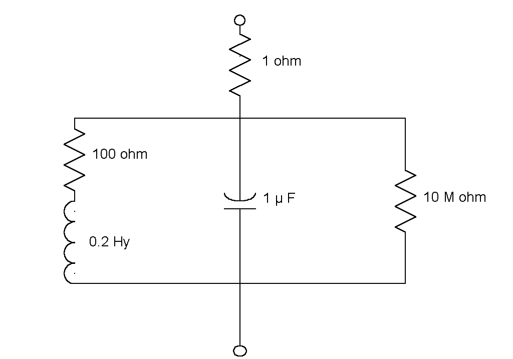
Figure 10-6: Example of an electrical circuit
10.9.1 Descriptions of electrical circuits
Suppose, an electrical engineer wants to design a system for the evaluation of two-terminal electrical networks, such as given in Figure 10-6. As components he uses resistors (R), capacitors (C) and inductors (L). To express the network in an expression he also needs the Series function to indicate that two components are connected in series. Similarly, the function Parallel indicates parallel connection. The impedance of the circuit as shown in Figure 10-6 can now be described by:
R1 = 1.0; R2 = 100.0; R3 = 10.0E+6; L1 = 0.2; C1 = 0.000001;Circuit (Omega = Numeric) -> Impedance; Circuit (Omega) = Series ( Resistor (R1), ( Parallel (Series (Resistor (R2), Inductor (L1, Omega)), (Parallel (Capacitor (C1, Omega), Resistor (R3))))));
Here Omega is the angular frequency in radians per second, or as a formula: 2.0 * pi * frequency.
10.9.2 Impedances of electrical components
Before the impedance of the circuit can be computed, the impedances of the components of a circuit have be to be defined. The impedances of resistors, inductors and capacitors are expressed by the following definitions:
Resistor (Ohms = Numeric) -> Impedance;
Resistor (R) = Impedance (R, 0.0);
Inductor (Henries = Numeric, Omega = Numeric) -> Impedance; Inductor (L, Omega) = Impedance (0.0, Omega * L);Capacitor (Farads = Numeric, Omega = Numeric) -> Impedance; Capacitor (C, Omega) = Impedance( 0.0, -1.0 / (Omega * C));
The impedances of the Series and Parallel functions are:
Series (Impedance, Impedance) -> Impedance;
Series (Z1, Z2) = Z1 + Z2;
Parallel (Impedance, Impedance) -> Impedance; Parallel (Z1, Z2) = (Z1 + Z2) / (Z1 * Z2);
With these five basic functions all two-terminal networks can be defined.
10.9.3 A Component for Complex Numbers
To compute impedances, the standard method is to use complex numbers. So, we will introduce a software component for complex numbers (see Figure 10-7).
component ComplexNumbers;
 type Complex;
      Complex (Real = Numeric, Imag = Numeric) -> Complex;
      Complex + Complex -> Complex;
      Complex - Complex -> Complex;
      Complex * Complex -> Complex;
      Complex / Complex -> Complex;
begin
      Complex (R, I) = Complex:[ R; I ];
      C1 + C2 = Complex (C1.R + C2.R, C1.I + C2.I);
      C1 - C2 = Complex (C1.R - C2.R, C1.I - C2.I);
      C1 * C2 = Complex (C1.R * C2.R - C1.I * C2.I,
                         C1.R * C2.I + C1.I * C2.R);
      C1 / C2 = [ D = C2.R ** 2 + C2.I ** 2;
                  Complex ( (C1.R * C2.R + C1.I * C2.I) / D,
                            (C1.I * C2.R - C1.R * C2.I) / D) ];
end component ComplexNumbers;
Figure 10-7: Example of a component for complex numbers
In order to use the property of referential transparency we defined complex numbers by means of immutable descriptors.
To make the connection between impedances and complex numbers we need to define in front of the five basic network functions the following declarations:
type Impedance = Complex;
Impedance (Numeric, Numeric) -> Impedance;
Impedance (R, I) = Complex (R, I);
10.9.4 A Component for computing Impedances
Now we have all the necessary ingredients for defining a general component for the computation of impedances (see Figure 10-8).
component Impedances;
 type Impedance = Complex;
      Resistor (Ohms = Numeric) -> Impedance;
      Inductor (Henries = Numeric, Omega = Numeric) -> Impedance;
      Capacitor (Farads = Numeric, Omega = Numeric) -> Impedance;
      Series (Impedance, Impedance) -> Impedance;
      Parallel (Impedance, Impedance) -> Impedance;
      Omega (Frequency = Numeric) -> Numeric;
begin
      Impedance (Numeric, Numeric) -> Impedance;
      Impedance (R, I) = Complex (R, I);
Resistor (R) = Impedance (R, 0.0); Inductor (L, Omega) = Impedance (0.0, Omega * L); Capacitor (C, Omega) = Impedance ( 0.0, - 1.0 / (Omega * C)); Series (Z1, Z2) = Z1 + Z2; Parallel (Z1, Z2) = (Z1 * Z2) / (Z1 + Z2); Omega (Frequency) = 2.0 * 3.14159265 * Frequency; end component Impedances;
Figure 10-8: Example of a component for impedances
The impedance of a circuit for a given frequency can now be computed after setting up the following configuration:
type Numeric = real;
use ComplexNumbers;
use Impedances;
We will start with some very simple examples, such as computing the impedances of two resistors in series and parallel:
Series (Resistor (20.0), Resistor (30.0))?
Complex:[ R = 50.0; I = 0.0]
Parallel (Resistor (20.0), Resistor (30.0))? Complex:[ R = 12.0; I = 0.0]
Our next example is to compute at a frequency of 300 Hertz the impedance of an inductor of 0.5 Henry which is parallel connected to a capacitor of 1 micro Farad:
L = 0.5; C = 1.0E-6;
Parallel (Inductor (L, Omega (300.0)), Capacitor (C, Omega (300.0)))?
Complex:[ R = 0.0; I = -1213.7061875867]
Our next example is the circuit of Figure 10-6:
R1 = 1.0; R2 = 100.0; R3 = 10.0E+6; L1 = 0.2; C1 = 0.000001;Circuit (Omega = Numeric) -> Impedance; Circuit (Omega) = Series ( Resistor (R1), ( Parallel (Series (Resistor (R2), Inductor (L1, Omega)), (Parallel (Capacitor (C1, Omega), Resistor (R3))))));
Circuit (Omega (300))?
Complex:[ R = 839.3766753887; I = 756.4975057023]
And this concludes our exercise.
- A component is a self-contained software building block with a well-defined interface with its outside world.
- A software component consists of two parts:
* an interface-section
* an implementation-section
- A component provides a number of services to its clients. The services a component provides are specified in its interface-section.
- The definitions in an implementation-section are encapsulated.
- Components may be based on other components.
- Use directives are used to invoke components.
- Components can be tested in interactive sessions.
- Components based on mutable objects are behaving differently from components based on immutable objects.
- Referential transparency is an important property of names referring to immutable objects.
The example of electrical circuits has been adopted from Winston(1984).
| Part 1: Language Description | Chapter 10: Components |